Harry Liuhan

April 10th

A perfectly clean graph can describe the wrong motion. That is the unsettling part of aliasing: the problem need not look like noise, missing values or a broken sensor. Every recorded point can be correct while the oscillation inferred from those points is wrong.

Suppose a sensor records ten measurements per second. Consider two signals, each with amplitude one: a cosine oscillating three times per second and another oscillating seven times per second. At the sampling times, their values are identical. If n numbers the measurements, the phases are 0.6πn and 1.4πn. The second can be written as 2πn minus 0.6πn; cosine’s periodicity and symmetry then make the sampled values equal.

This gives a rather striking imaginary experiment. Feed the two oscillations into identical recording systems, export the data, and ask someone to identify which file came from which signal. With those samples alone, they cannot. A more sophisticated analysis cannot distinguish two inputs that produced exactly the same observations.

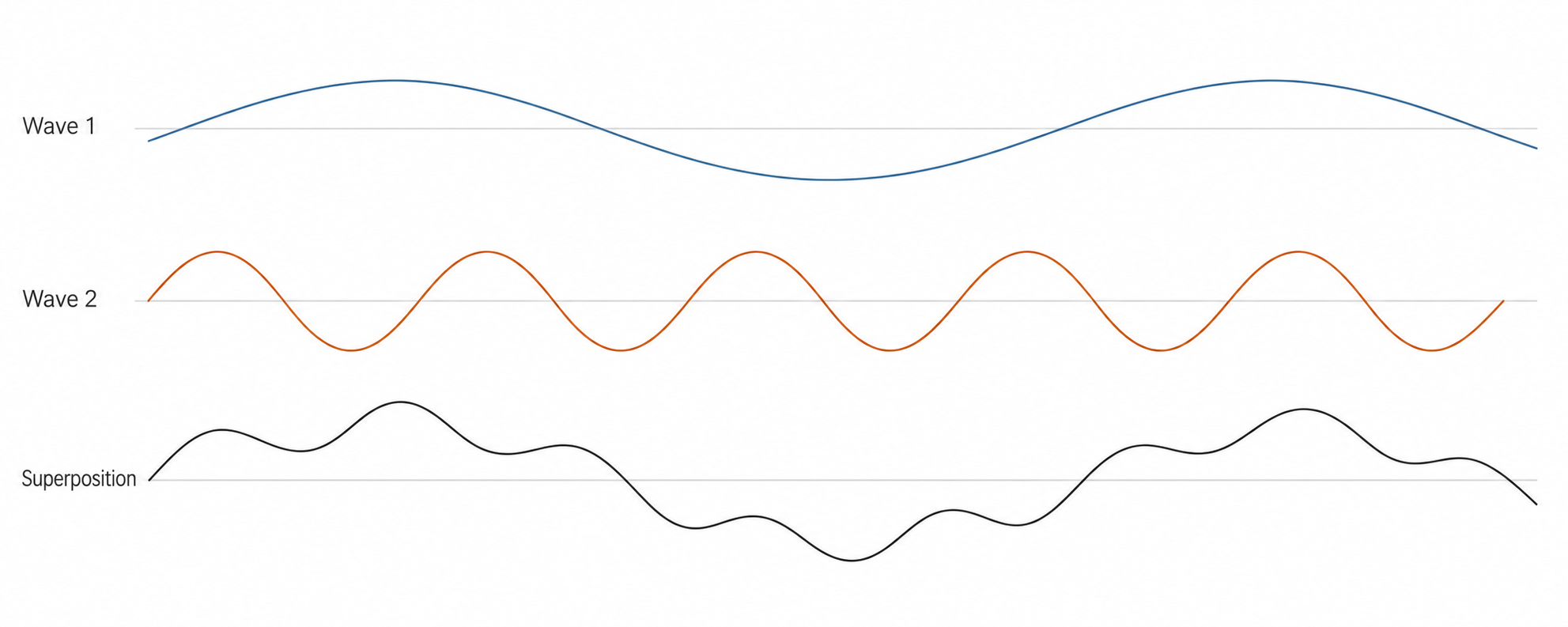
The sampling theorem tells us how to avoid this ambiguity under specific assumptions. For a signal containing no frequencies above a known limit, an ideal sampling rate greater than twice that limit allows reconstruction. Real instruments also need suitable filtering before sampling, so unwanted high frequencies do not fold into the measured range. [1]

There is a second limitation that is easy to confuse with sampling rate: recording duration. A conventional discrete Fourier transform has frequency-bin spacing equal to one over time (recording duration). A ten-second record gives bins which are 0.1Hz apart; a hundred-second record gives 0.01Hz. Faster sampling and longer recording solve different problems. Zero-padding can make the displayed spectrum smoother, but it does not add observations.

For a hypothetical vortex-shedding experiment, I would therefore ask two separate questions. Have I sampled quickly enough to capture the relevant oscillations? And have I watched for long enough to distinguish nearby frequencies? A short, densely sampled record might answer the first while failing the second. A long, sparsely sampled record could do the reverse.

I like that this turns data collection into a mathematical decision before any data exist. Choosing when to observe determines which explanations will remain distinguishable afterwards. The Fourier transform is powerful but cannot recover distinctions that the measuring process erased. A sharp peak deserves attention; it also deserves a look back at the clock that produced it.

[1] Texas Instruments — An introduction to the sampling theorem